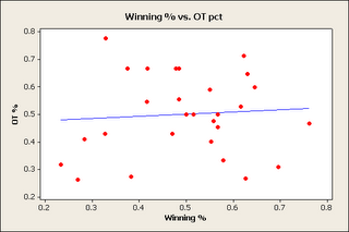
In the last article I concluded that: “I have good reason to conclude that overtime occurs randomly given any two team and that the results once in overtime are completely random.” My analysis before was focusing on global overtimes in order to know how to predict what games will go to overtime in order to make my point predictions more accurate. The graph below shocked me the most during my previous analysis, that is to say teams with a lot of regulation wins were unable to perform better in the overtime session, this is both shootouts and the 5 minute four on four. Of course I wrongly concluded that this suggests the results are random, however I think most readers will agree that if skill doesn't determine who wins, then what on earth does win?
Randomness
Randomness naturally creates clusters and anomalies these should be expected. The question to ask is "are there too many anomalies?" Now a season is only 82 games and there are 30 teams, most of which see around 20 overtimes. One of the beautiful things about this analysis is that we know the distribution for random binary variables. That is to say that the mean = probability (p) and the standard deviation sqrt(n*p*(1-p))/n [n = number of events]. If a variable is perfectly random with equal chance for each side to win, then we obviously expect the probability to be 50%, which suggests that the error is sqrt(n)/(2n) or 50%
± sqrt(n)/(2n). So if you were to flip a coin 4 times you'd expect to get heads: 50%
± 25%, for a 95% confidence interval of (0%, 100%), of course this is a 100% confidence interval (you can't ever get above 100% or below 0%, so I'm 100% sure that 4 coin flips will land in that range) as a result of problems with approximating the normal distribution with the binomial distribution with small n.
In the NHL you can always find teams that fall outside if the normal 95% range due to the fact there are 30 teams, and if I'm 95% confident that each team is in this range than I could say that 5% should be outside of this range so 1.5 teams should be on the outside on average, so 2 teams outside this range is actually reasonable. If you wanted a range that includes all teams you'd want a 99% or 99.5% range (3 standard deviations).
Modeling the Overtime
I could use theory to analytically calculate the values for winning in overtime, but it's often easier to write a script to simulate the results. First I simulated the 4 on 4 assuming team A was 9% better than team B. So team scored at a rate of 1.2 goals per 20 minutes and team B scored at a 1.1 goals per 20 minute rate [Defense is ignored]. These numbers accurately reflect the actual scoring in the overtime. I simulated 50,000 times so the results should be
± 0.2%. The result: A team who is 9% better wins 52% of the time. The shootout relied on skill a little more, that is to say a team who has a 10% better shooting percentage (whether this comes from shooting or goal tending tending is irrelevant) results a team who is 10% better than team a wins 54% of the time. So shootouts should correlate about twice as much as overtime. There is only a 50% chance to make it to a shootout once you get to the overtime. As I mentioned before there is correlation between winning in OT and winning in regulation, but it's not significant. This often means that given more data there could be a relationship (this is always possible), but we are limited because there is only 1 season of data for this year. There is a more significant relationship to winning in shootout over the four on four portion as predicted by this simulation. Of course if you look at the variables and do regression nothing comes out as important, for example: save percentage doesn't appear to matter in the shootout. So we have theory that say better teams should win, but they don't appear to, but even if they did win at 52% it would be hard to detect (and having 2% error in a prediction algorithm isn't that bad).
Actual Results
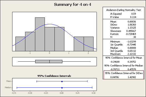
The easiest way to test if data is random is compare it to what true randomness would predict. Each team has a given percentage of winning and compare that to how it would "normally" distribute if it were random that is to say calculate a z-score = 2*(team score - 0.5)/(sqrt(n)/n) and then plot the z-scores. [error/standard deviation] For example Dallas' 12-1 works out to 2*(12/13-0.5)/(sqrt(13)/13) = 3.05. 3. In other words the error is 3 standard deviations away from average, which is extremely rare (0.25%), but the probability that one team is 3 standard deviations away in a season is 8%, which is low, but not unreasonable. So Dallas probably was good and lucky. Not sure how physiology plays into all this: that is to say, if you go into Dallas knowing they're 11-1, you will think you will lose and hence you lose. Once you have a set of z-scores for each team you can plot them. If they're perfectly normal (mean = 0, standard deviation = 1) then you can conclude that the variability is identical to that of randomness (whether this means it's random is of course not determined). Minitab creates nice summaries of this data and they include the "standard deviation of the standard deviation". Like all statistics neither the mean or standard deviation is known and we must estimate both and with every estimate there is error and so the standard deviation has error just like the mean, now if this error doesn't include 1 (the value required for randomness) at a statistically significant level I can conclude this data is statistically significantly not random, however if it does include 1 that would mean that I must not reject* the possibility it's the same as randomness. So below are these statistics and in the red box I have a 95% confidence interval for the standard deviation.
Now if you understood any of that you would have noticed that the 4 on 4 and overtime in general included 1 and the shootout did not. That is to say there was statistically significantly more variability in the shootout than we would expect if it were random. So Dallas probably wasn't 3 standard deviations from their actual score (maybe 2.5 or 2, who knows), but the others were too close for this small data set to determine if it is random or not (I'll will add this years data at the end of the season and see if it becomes significant). Of course all these standard deviations appear more variable than randomness and it's only on the margins that we see
My Predictions
The important variable: overtime, includes 1 and as such there is insignificant evidence at this point to consider overtime determined by anything other than randomness, since overtime is what I care about (who gets the extra point) and not if the game is a shootout or won in the 4 on 4 I have choose to use a random variable to predict overtimes. I will again remind the readers that not only does overtime have very similar properties to randomness it doesn't correlate to skill, so bad teams win just as often as good teams do. This means that there is no useful way to actually predict who will win the OT even if I knew it weren't random. Does this mean that overtimes are the same as a random variables: absolutely not they are extremely complicated, have 18 skaters, a goalie, a coach (and assistants), referees, dynamic wind, air and ice variables not to mention physiological factors, however
at this point, based on the data available to me, the best model is a random variable.
Challenge to Everyone
I challenge the readers to prove me wrong, that is to say to show that there exists a statistically significant (95% confidence) variable that can predict the overtime results.
*Hypothesis tests:Has two hypothesis:
Null hypothesis claim initially assumed to be true [the data is random]
Alternative hypothesis: a assertion that is contradictory to the Null hypothesis [the data isn't random]
When we do the test we have two options:
Reject the Null hypothesis in favour of the alternative [reject: "the data is random" for "the data isn't random"]
or
Do not reject the Null hypothesis and continue with the belief that our initial claim was true ["the data is random"]
This does not prove the data is random, simply that its not different enough from random that we should conclude otherwise. This is exactly what I'm saying: there's insufficient evidence for me to use anything other than a random variable in my model.
Due to the nature of this site I'm often a little loose on the concept of "not rejecting" and"accepting" (they're different), just because this isn't supposed to be perfectly formal.


 Summary of the Graphs
6 comments:
TMS: PCT = OTS/GAMES [GOALS/GAMES]
BxB: 30 = 45/150 [6.2] Z=1.951
MxM: 22.5 = 27/120 [5.8] Z=-0.052
TxT: 23.7 = 31/131 [5.9] Z=0.26
BxT: 19.3 = 48/249 [6] Z=-1.369
MxT: 20.4 = 63/309 [6] Z=-1.009
BxM: 24.4 = 66/271 [5.8] Z=0.634
Confidence interval for the standard deviation:
(0.76, 2.98)
Includes 1, there's nothing here that helps
1. You counted the Bottom x Bottom, Mid x Mid, Top x Top twice.
2. Does this "score" really measure skill? [I have no knowledge of method], so I cant even reproduce the results.
3. score = f(W,L,OTW,OTL,SOW,SOL) and now you're doing (OTW+OTL+SOL+SOW)=g(score), that's cheating.
4. The bottom teams see MORE scoring
I'm not saying they're random, I'm saying the best way to model them at this point is using a random variable as they don't correlate significantly with possible variables:
Does this mean that overtimes are the same as a random variables: absolutely not they are extremely complicated, have 18 skaters, a goalie, a coach (and assistants), referees, dynamic wind, air and ice variables not to mention physiological factors, however at this point, based on the data available to me, the best model is a random variable.
I haven't convinced myself that overtime isn't based on skill, but simply that the skill it's based on is currently undetectable because of error.
Score = Power Rank. And the problem is: Your algorithm looks at overtime results to get a power rank and then you uses power rank to determine the number of overtimes...
The interval 90% occurs at Z=1.6 and this would still result in the above data including the standard deviation on 1.
The p-value for this data is 13%.
However, you can't just choose a confidence level after looking at the data.
Sure I see room for future considerations as all statistical analysis should conclude, but at the present time I lack the information. And I suspect people would be hard pressed to find something that correlates significantly.
Sorry I forgot to mention.
GOALS = goals scored by home team + goals scored by away team [only during periods 1,2,3] Basically the total number of goals scored in the games, so divide by games you get the average goals scored in these games.
GOALS:
EG
Bottom 10 vs Bottom 10 Played 150 games together 46 went overtime.
In the 150 games they played together there were 925 goals scored by both teams in the first three periods.
It's funny, but I calculated this years results [using my Colley Matrix to rank teams]:
BxB: 11.8 = 4/34 [5.824] Z=-1.979
MxM: 23.5 = 8/34 [6] Z=0.114
TxT: 27.6 = 8/29 [5.69] Z=0.589
BxT: 21.1 = 15/71 [5.465] Z=-0.325
MxT: 22.4 = 15/67 [5.791] Z=-0.061
BxM: 22.4 = 13/58 [5.931] Z=-0.052
BxB from both seasons would make:
50/184 = 27.1% Not so significant anymore.
Also, it interesting if you break the season into three parts only one part is significantly different and in fact an a more significant anomaly occurs with good vs. bad in the first 410 games (-3.5 standard deviations) however the other 17 points are more normal
Also, on Wednesdays 27/157 games went to overtime for 17% (a difference of ~6%) or Z=-1.83.
Post a Comment