Home Team Advantage

“I do think that opposition and line matching makes a big difference. The biggest argument for that claim is that home teams win 55% of the time. That is a fairly significant advantage. And what is the biggest advantage that home teams get? A greater ability to match lines because the road team has to put their line on the ice first” (David Johnson). On first glance I agreed that 55% home win percentage is significant (this is constant over seasons with a range of about half a percent) should indicate that the ability to change last, the only significant difference given to home team, should give the home team this advantage. A further analysis shows that goal for increase by 10% at home and goals against fall by 10%. There appears to be two parts to this question: what increases scoring at home, what decreases goals against? It should be noted that goals for the home team equal goals against the away team. There were a total of 3986 goals accredited the home team (These include 1 extra goal for the worthless SOWer, but this wont be significant) and 3602 accredited to the away team for a total difference of 384 goals.

Before focusing on the possible differences I should state the NHL wants the home team to win, probably because if a new fan is in the stands of a win they’re more likely to return than if there’s a loss. So for example the average number of rest days for the home team is 2.4 days rest average and away teams have 2.2 average days of rest (back to back games are counted as 1 day rest). There is a similar home team favored schedule in 2005-2006 as well: 11% of home team’s games are back to back, where 26% of away team’s games are back to back.

Power Play.

It’s interesting to note that there are an additional 405 penalties given (only minors) to the away team (1/3 per game) (8199 vs. 7794), might sound like a little, but this should work out to around 60 goals. If you just look at the more subjective calls (the ones they can ignore) you get a more significant difference of 390 (6457 vs. 6067), which is a lot larger as a percentage. Interesting these power plays resulted in 1382 power plays goals for home and 1162 for the away team (difference of 220), which suggests this problem is a little more complicated. A way a referee can get the home team more goals without giving more penalties is to give them a little closer together so as to result in “5 on 3”s. The home team scored 266 “5 on 3” goals vs. 189 “5 on 3” goals for the away team. There’s really no good reason for this, because each team will be playing their best available. This accounts for 77 of the 220 (leaving me with 143, when I would only expect 60). One could argue that strength of opposition can affect whether a player takes a penalty. Whether this is mandated by the NHL or simply the result of the fans would be hard to determine unless a ref outright stated it to the media, but either way the home team is getting a lot more “5 on 3”s (or scoring with them at much high rate).

The Backup

On the surface most people wouldn’t expect this to be a factor, but teams want to give a good show to the home team so when possible teams shift their secondary goaltending into away games. In fact the ratio of home to away is quite significant as the backups play 20% more games away then at home for about 3 extra games away than at home (there's a large variation between teams due to the fact it's hard to write an algorithm that picks the #1 goaltender). If you consider the backups save percentage to be 1.5% (.905 vs. .890) worse than a primary goalie and consider there are about 100 shots on goal for the backup away vs. at home in those three games, or about 1.5 goals per team or 45 goals over the course of the season (Approximately 15 on the power play and 30 at even strength). It’s interesting that Edmonton went the entire season without a definitive number one goaltender and they’re winning percentage doesn’t change for home or away games.

Even Strength

If the strength of opposition was significant, it should be most significant at even strength. There’s a 145 goal differential favoring the home team (or 6% difference), of course I brush this aside by stating the standard deviation of goals is 50 (±100) and if you compared these two distributions simultaneously you’d see no significant difference (73 < style=""> Of course 30 of these 145 can be accounted with goaltending alone (30 * 2 due to the fact that removing goals for from the home team lowers the goals against for the away team), reducing it to 85 (which is within one standard deviation of a mean of 50%) or 3.8%. This would result in a 51.8% winning percentage for the home team, which I wouldn't consider near as significant as 55%.

Difficult to Quantify

Of course this doesn’t cover aspects such as knowledge about your ice, sleeping in your own bed (positive or negative?) also one should consider Travel, which I’ve never seen had an affect on winning percentage. Players likely want to win for their home fans more than the away fans, they might plan a different style that results in more losses on the road (whether it’s logical or not). Detroit is likely a good example here; they won at 70% on the road and 67% at home. Detroit won the division easily and was top in the conference by a margin of 12 points (6 wins), Detroit had a much smaller incentive to play well (the fans wont complain about 67%). Ever tried to quantify goals called off (early whistle) that favor the home team? I'm sure the readers can think of a number of other area to include here, but this is a start.

Conclusion

To say there’s no such thing as line matching would be crazy, almost every coach attempts some protection and some abuse of players to maximize their goal differential, but whether this affects the outcome to a significant extent is rather subjective. Either way a 2% change in player scores would be indistinguishable from error and including the strength of opposition would likely make the model more complicated then the benefits of the added information. At this point it would be much more beneficial to be able to understand the dynamics of line mates rather than opposition as it would provide much more insight into the game. Also, If you consider that the time sheets have error (human error) in reporting ice time, strength of opposition would be near impossible to determine because the error would dominate the possible information.

Strength of Opposition II

I still have my doubts about strength of opposition. I went through every team picking out the top forward on the team (mostly based on points and even strength ice time). At this point my list could be quite imperfect. Using simple statistics I was able to calculated expected ice time with another player. For example the probability player 1 is on the ice is 25% and the other player is 33% suggests that if those two variables are random and independent they would spend 8.25% of the game together, so if a player plays more than that against the top players then we could say he’s getting a tougher opposition. One can easily compare the ratio of actual percentage together vs. real percentage together, so for example if the above players actually spent 10% of the game together then they would’ve spent 20% more time together than expected.

So using a “measuring” player (not sure I have the best set yet) from each team I can sum up total even strength time, total time by a given player and then sum up the total time of my measuring player. I get an average of the percentage of even strength time of the player and top opposition percentage. I can simply compare that to the expected time vs. actual time. The results were a little surprisingly useless the most “abused” players only received 4% more difficult opposition (all from same team: Florida). The most protected player was Ryan Sutter of the Nashville Predators with a rating of -5%, this would suggest his statistics are off by -5% multiplied by the relative difference between the top players and average players (if 3 times better than average players than the easier opposition is making their statistics appear 15% better than they should be). However 95% of the players are within 2% of 1, so most players are seeing tougher opposition 2% more often than expected (only affect their statistics by 6% if top players are 3 times better than average). This would be indistinguishable.

I'm not saying people don't try, in fact Bourdon for example has had the easiest opposition on the Canucks. It's just tough to get significant scores when the opposition is trying to do the opposite as you are (get good players out against your bad players) and you have to deal with the physical limitations of your personnel. I have never seen convincing proof that this exists. Doesn't mean I wont keep looking, but I think I can at least attempt to build a model without worrying about opposition and just worrying about teams lines and strength of the opposing team.

Early Predictions

I’ve been having some fun predicting the outcome of the season with very little data. Like many readers realized these predictions aren’t really predictions as such as they have way too much error and make predictions all people know wont happen, like Phoenix getting less than 30 points. This is largely because one game’s goals against can significantly affect the average (9 goals against in one game increases the average over 9 games by 1 goal, which is a lot in terms of winning percentage). So I needed a formula to get a more accurate average for teams with anomalies in their data set (results that should only happen 1% of the time, occurring in 10% of their games). The goal is to scale game’s scores that are too many standard deviations away from the team’s average to a smaller part of the team’s average.

The nice thing about these predictions is that in general I know the standard deviation for goals against (the problem data), if a team has a game that’s more than 2 standard deviations away from their average then that game, should only happen about 4 times in a season and 3 standard deviations once every 5 seasons. In hockey goals against occur with an average of 2.85 and standard deviation of 1.7. Thus an average team should have 8 games in a season with 5 or more goals against, a bad team probably 16. So I take any game that’s beyond 1 standard deviation and give it a smaller weight. For standard equal weights you multiply every term by 1/n, for my weights I multiply by some constant c_i/(Σc_i), where c_i = 1 if within 1 standard deviation of the average and c_i = √(1.7/μ– ga_i) otherwise. The square root increases the amount of focus it puts on outliers, I used it because it produces slightly better results.

The neat thing about predictions in sports is that if you can define some algorithm you can test it on past data (and hope it works in the future). So, since I have 2005-2006 data, I can test this algorithm on the first few games of that season and see how well it performs. The first test any sort of regression should do is how much error does an average have. The total sum of squared error for the average is 7927, my original model actually increased the error (one team had error of 68 contributing to almost half of the total error). So I reapplied my normalizing algorithm mentioned above and got a sum of squared errors to be 5317, or 72% for an r² of 33%. Or I could say with 12% of the games I was able to explain 33% of the final variability. 9 teams were within 5 points of their predictions (almost a third), and 19 were within 10. The standard deviation was 13 (for a ± 26 confidence interval 95% of the time), which is better than the 20 I predicted from before. The worst prediction was Dallas who got 38 more points than predicted (they had a lot of goals against early on, but won games) accounting for 27% of my error. While this is a regression style analysis, the prediction is not based on a regression, but simply on the assumption that goals for and goals against correlate with winning (which is known).

Problem with my predictions this year and 2005-2006 predictions is that there appears to be a more competitive start to the 2005-2006 season than this year. So the best prediction was 109 points and the lowest was 60, creating reasonable minimums and maximums. This season teams don’t seem to want to be competitive there are a significant number of good teams to start this season: Dallas, Anaheim, Ottawa, and Atlanta not to mention the bad teams: Philadelphia, Chicago, Columbus, and Phoenix. The question of course is whether this season will be less competitive than past season (possibly a direction of the new CBA – I’ll look into later). What I’m basically trying to say is that the best algorithm of 2005-2006 won’t produce the best results for 2006-2007, but they should be useable.

So without further ado, here are the 2005-2006 results.

WEST:

Team PTS EPTS ERR Detroit Red Wings 124 102.554 21.4 Dallas Stars 112 74.1465 37.9 Calgary Flames 103 89.7303 13.3 Nashville Predators 106 89.1933 16.8 San Jose Sharks 99 98.1116 0.9 Anaheim Ducks 98 91.138 6.9 Edmonton Oilers 95 89.3213 5.7 Colorado Avalanche 95 91 4.0 Vancouver Canucks 92 90.5752 1.4 Los Angeles Kings 89 88.5126 0.5 Minnesota Wild 84 85.8979 1.9 Phoenix Coyotes 81 89.3955 8.4 Columbus Blue Jackets 74 80.4389 6.4 Chicago Blackhawks 65 83.1687 18.2 St. Louis Blues 57 77.0534 20.1

EAST:

Team PTS EPTS ERR Ottawa Senators 113 107.501 5.5 Carolina Hurricanes 112 102.183 9.8 New Jersey Devils 101 79.0032 22.0 Buffalo Sabres 110 92.838 17.2 Philadelphia Flyers 101 92.983 8.0 New York Rangers 100 98.7356 1.3 Montreal Canadiens 93 88.2429 4.8 Tampa Bay Lightning 92 98.0173 6.0 Toronto Maple Leafs 90 80.0578 9.9 Atlanta Thrashers 90 84.3788 5.6 Florida Panthers 84 94.902 10.9 New York Islanders 78 81.3242 3.3 Boston Bruins 74 89.3152 15.3 Washington Capitals 70 70.1098 0.1 Pittsburgh Penguins 58 80.2557 22.3

Of course I cannot predict or for that matter know what teams will do to solve problems early on. Boston for example (projected for 89 points) traded their top forward to San Jose (predicted exactly due to bad prediction for Dallas [over predicts San Jose to win games vs. Dallas] and Joe Thornton [Better player, better team] compensated each other). This may not be all that useful at this point, but it’s a start. Unlike most predictions I’m at least testing my hypothesis!

East

I always have a hard time following the East keeping track of the teams and players (30 teams are a lot of teams to keep track of), but these standing show quite nicely how these teams have done early on. Penguins and Thrashers are in the playoffs, New Jersey and Carolina are out. Rangers are in a bubble chased by Washington (we’ll see how long that lasts…) and New York Islanders (who would’ve thought)

# Name GP EPTS WD MP 1 Thrashers 8 142 98% 100% 2 Senators 7 122 57% 98% 3 Penguins 7 107 71% 91% 4 Sabres 8 106 19% 90% 5 Canadiens 7 105 18% 88% 6 Maple Leafs 9 96 6% 78% 7 Lightning 8 94 2% 73% 8 Rangers 8 85 14% 55% 9 Capitals 7 78 0% 37% 10 Islanders 8 77 8% 38% 11 Devils 8 73 6% 28% 12 Hurricanes 9 63 0% 10% 13 Panthers 9 59 0% 7% 14 Bruins 7 52 0% 5% 15 Flyers 8 41 0% 1%

Northeast

# Name GP EPTS WD MP 1 Senators 7 122 57% 98% 2 Sabres 8 106 19% 90% 3 Canadiens 7 105 18% 88% 4 Maple Leafs 9 96 6% 78% 5 Bruins 7 52 0% 5%

The one division I can follow because it is over half Canadian. Senators are still expected to win the division despite their low initial point totals. This is another division that could bring 4 teams into the playoffs. Certainly the Maples Leafs can’t miss the playoffs two years in a row. And the Bruin’s appear to have lost all ability to succeed after losing Thornton and will wind up in the bottom of this group. The Bruin’s may have made a mistake signing a goaltender long term without accurate data.

Atlantic

# Name GP EPTS WD MP 1 Penguins 7 107 71% 91% 2 Rangers 8 85 14% 55% 3 Islanders 8 77 8% 38% 4 Devils 8 73 6% 28% 5 Flyers 8 41 0% 1%

With Malkin and Crosby playing for the Penguins they appear to have enough scoring. The penguins also seem to have come to their sense and use Fluery as their number one goaltender to keep the goals down. If Lundqvist can play like he did last year the New York Rangers should give the Penguins a tough battle to keep this spot. As I mentioned in the above it’s interesting to see the poorly managed Islanders playing well, we’ll see how long it lasts.

Southeast

# Name GP EPTS WD MP 1 Thrashers 8 142 98% 100% 2 Lightning 8 94 2% 73% 3 Capitals 7 78 0% 37% 4 Hurricanes 9 63 0% 10% 5 Panthers 9 59 0% 7%

The division I find boring simply because all the teams are so bad (Yet they find a way to win the Stanley Cup and crash and burn the next year). Carolina went from best to worst, not because they can’t score, but because they can’t stop goals from going in. The Thrashers seem to continue to roll they’re on last year with excellent goaltending and a ton of scoring they should have no trouble doing well and likely winning the division. Washington has done well (largely due to Johnson and not Kolzig). They’ve kept their goals against down and can score enough goals to be competitive in the easiest division in hockey. Carolina dumped their goaltender Gerber in favor of their playoff hero Ward and it hasn’t worked out too well for them. Ward didn’t win the cup because of his stellar performances, but because the team got a lot of goals for their goaltender. Florida hasn’t gotten it together, their goaltending has been average (Auld) and below average (Belfour) and they cannot score goals.

I should note: (all based on a model with 10,000 iterations).
WD - Probability of winning division
MP - Probability of making the playoffs
EPTS - Expected points based on a statistical prediction

West

Arguably any statistics at this point in the season don’t say all that much about the final outcome of the season. As I stated in a previous post one game error for winning percentage can be approximated to around 36%, with a crude sqrt(n)/n approximation I can say that 8 games in works out to 13%. It should more importantly be noted that 13% is equivalent to around 20 points, so teams have 20 points worth of error, or I could say I expect Vancouver to get 95 points ± 40 (95% confidence interval), which doesn’t tell you all that much about how the Canucks will do (bad predictor), but it appears the NHL is settling down to some sort of balance. The Ducks have taken over the west (for now) as a very dominant team, and Detroit continues its dominance within their division. Calgary is a bit of a shocker, but they’re not scoring and they’re not preventing goals so they’re hitting rock bottom and they will have a hard time competing in the Northwest division.

# Name GP EPTS WD MP 1 Ducks 7 145 66% 100% 2 Stars 8 137 33% 100% 3 Red Wings 8 112 83% 92% 4 Oilers 7 111 42% 89% 5 Sharks 8 109 1% 90% 6 Wild 8 109 35% 87% 7 Avalanche 8 97 11% 69% 8 Canucks 9 95 11% 62% 9 Kings 8 93 0% 56% 10 Predators 8 87 15% 44% 11 Blackhawks 8 62 1% 5% 12 Blues 8 59 1% 4% 13 Flames 7 55 0% 3% 14 Blue Jackets 6 42 0% 1% 15 Coyotes 8 25 0% 0%

What’s neat is you can already see the playoff battles setting themselves up with Nashville and L.A. trying to steal the spot from Vancouver. Coyotes unless they make drastic changes have a 0% chance of making the playoffs, and the Blackhawks, Blues, Flames and Blue Jackets all have less than or equal to 5% chance of making the playoffs (which to a statistician is about as good as no chance). It might be confusing to some that Detroit’s 7 points gets them into 3^rd. I should say I’m looking that expected goals not actual goals to predict future games and Detroit may have only scored 20 goals, but they’ve played at a level that should get 25 goals. This could be because of better goaltending on the other teams or just “bad luck”. The Avs are another good example scoring 24 goals (and allowing 27), but their expected goals are 32 or (4 goals per game, I doubt they’ll keep that up).

# Name GP EPTS WD MP 1 Oilers 7 111 42% 89% 2 Wild 8 109 35% 87% 3 Avalanche 8 97 11% 69% 4 Canucks 9 95 11% 62% 5 Flames 7 55 0% 3%

Northwest

Every team is good and every team is not quite great. You can see the battle for the division is by no means determined, but mostly a battle between the Oilers and Wild. While unlikely my number crunching is predicting 4 of the Northwest teams to make the playoffs this season, largely due to the poor performance of the Central division (unable to get 2 teams in). If the Flames maintain their level of play they performed in the first 7 games of the season they have a 3% chance of making the playoffs. It would appear that the games within the division will be critical for success in this division.

# Name GP EPTS WD MP 1 Red Wings 8 112 83% 92% 2 Predators 8 87 15% 44% 3 Blackhawks 8 62 1% 5% 4 Blues 8 59 1% 4% 5 Blue Jackets 6 42 0% 1%

Central

I wonder when this division will get competitive. A lot of people may have considered Chicago a much better team with Havlat (now injured) playing so well, but their goals against keep adding up and keeping them held back. The Blues keep allowing goals against as do the Columbus Blue Jackets. I expect that the Predators will make the playoffs despite what this shows, Vokoun probably isn’t as good as he played last year, but he’s better than how he started this year. Detroit, despite being an average team, should have no trouble winning the division.

# Name GP EPTS WD MP 1 Ducks 7 145 66% 100% 2 Stars 8 137 33% 100% 3 Sharks 8 109 1% 90% 4 Kings 8 93 0% 56% 5 Coyotes 8 25 0% 0%

Pacific

The pacific division is a very dynamic division, and Phoenix would be a much better team this year if they didn’t have to play Dallas and Anaheim 8 times in one season. The three top teams are very dominant at this point it’s hard to say who’ll win this division. Anaheim’s defense certainly bodes well for them and they have enough scoring to win games. Dallas can score, but their defense is questionable and it appears as though Turco is outplaying his average at this time. San Jose is great at scoring as well, but their goaltending is questionable, not that is really matter when you can score. In any other division the Kings would be a competitive team, but they’ll likely be playing golf early this year. It’s hard to imagine a scenario that would get Phoenix into the playoffs, just hope you win 6 or 7 games out of the 8 you play them if you’re in this division.

If you like these standings I up them periodically at my statistics website

I should note: (all based on a model with 10,000 iterations).
WD - Probability of winning division
MP - Probability of making the playoffs
EPTS - Expected points based on a statistical prediction

CBS SportsTicker shots vs. NHL official Shots

Shot comparison for http://www.nhl.com/scores/htmlreports/20062007/PL020008.HTM

MM:SS DIFF T1 FT T2 X Y NHL Player CBS Player 00:18:20 - 63 26 - DRAPER - - - - 100 37 21 - N. Lidstrom 00:17:08 -10 182 59 172 -48 -17 LIDSTROM N. Lidstrom 00:16:26 -7 221 36 214 10 19 ZETTERBERG H. Zetterberg 00:15:51 -11 260 54 249 45 -25 SALO K. Bieksa 00:15:30 -14 284 57 270 43 9 BIEKSA K. Bieksa 00:15:17 -7 290 42 283 8 9 NASLUND D. Sedin 00:15:07 -7 300 44 293 1 -7 SEDIN M. Naslund 00:14:12 - 313 10 - NASLUND - 00:14:12 -4 352 60 348 45 -20 LIDSTROM N. Lidstrom 00:12:14 3 463 58 466 44 -21 FITZPATRICK B. Morrison 00:09:05 - 516 61 - SALO - 00:09:05 -6 661 40 655 36 -10 LILJA K. Draper 00:06:29 -2 813 17 811 9 -11 DATSYUK P. Datsyuk 00:04:55 0 905 15 905 5 -3 DRAPER K. Draper 00:04:45 -7 922 63 915 45 -23 MITCHELL W. Mitchell 00:01:18 -12 1134 29 1122 17 -3 ZETTERBERG H. Zetterberg - - - 1144 36 -25 - M. Samuelsson 00:00:05 0 1195 13 1195 82 1 NASLUND M. Naslund 00:19:43 -3 1220 11 1217 11 10 COOKE M. Cooke 00:17:48 -13 1345 12 1332 40 6 LINDEN M. Naslund 00:17:35 -2 1347 28 1345 6 0 GREEN T. Linden 00:16:38 -20 1422 22 1402 15 -10 HUDLER J. Hudler 00:15:56 -26 1470 38 1444 36 -12 SEDIN H. Sedin 00:14:19 0 1541 47 1541 29 4 SALO S. Salo 00:14:11 -14 1563 13 1549 42 4 WILLIAMS P. Datsyuk 00:14:02 -10 1568 36 1558 10 -5 DATSYUK J. Williams 00:10:45 - 1631 30 - MORRISON - 00:10:45 - 1718 38 - ZETTERBERG - 00:10:45 -10 1765 17 1755 5 -9 SCHNEIDER M. Schneider 00:09:26 -6 1840 45 1834 35 4 SAMUELSSON M. Samuelsson 00:07:15 - 1848 16 - CLEARY - 00:07:15 -21 1986 14 1965 6 -3 HUDLER J. Hudler 00:06:59 -14 1995 12 1981 10 5 ZETTERBERG H. Zetterberg 00:04:05 0 2155 44 2155 14 18 ZETTERBERG H. Zetterberg 00:17:12 - 2373 12 - FRANZEN - 00:17:12 - 2494 66 - NASLUND - 00:17:12 -7 2575 50 2568 40 3 KRONVALL N. Kronwall 00:16:08 -5 2637 11 2632 38 -6 SAMUELSSON N. Lidstrom 00:15:41 - 2640 56 - LIDSTROM - 00:15:41 -3 2662 43 2659 31 -28 WILLIAMS D. Cleary 00:15:18 -6 2688 42 2682 26 18 SAMUELSSON M. Samuelsson 00:10:59 -27 2968 11 2941 -2 7 WILLIAMS J. Williams 00:05:40 - 3070 52 - MALTBY - 00:05:40 -17 3277 46 3260 43 0 LIDSTROM N. Lidstrom - - - 3310 34 15 - M. Samuelsson 00:02:40 -14 3454 68 3440 53 -15 SALO S. Salo 00:01:17 -22 3545 62 3523 39 23 MARKOV D. Markov

If anyone is wonder how you go about getting these shots to agree, this is how. I should note FT: represents the ft recorded in the NHL play-by-play. T1 is seconds since start of game from NHL official sheets, and T2 is seconds since start of game from CBS SportTicker. Diff is the difference between T1 and T2, X,Y is the cordinates of the shot supplied by CBS (I changed X a little though).

I recently discovered that the official sheets are not even close to 100% accurate with their shot information. For example, Green has a shot recorded 2 seconds after Linden's goal (early second perid), but Linden's goal came off a rebound from Green's shot (2 seconds before). The CBS SportsTicker didn't record Green's shot and the NHL recorded it wrong. Also watching the games it appears that the NHL records extra "marginal" shots that may have appeared to be going wide that the NHL later determined were "on net", how they figure this out I'm not sure. I haven't figured out which figure the NHL play-by-play shot distance or CBS X,Y cords are more accurate yet.

I'm not to sure how the SportTicker stuff is physically done, but it appears shots occur on average well before they physically occur. A good example is J. Williams shot at 2941 (CBS time), that the NHL recorded as 2968 (27 seconds later), that's one great prediction. So I'm curious exactly how they determine the times for the SportsTicker. CBS converts the SportsTicker data (GAME_TIME (Time in Period [As opposed to time remaining on clock])) to time remaining so they could have a mistake in their algoritm (or mine could be wrong). The times recorded of shots appear to be the release time as opposed to the stoppage in play time (when they hit the goaltender).

If anyone has ideas how to make things work better quickly that'd be great.

Error: Continued...

I felt this clip best represented peoples misconceptions of error. Numb3rs has mentioned these things before.

Obviously from my other discussions these things are quite important in terms of hockey statistics and sabrmetrics in general. Often once a statistic is proved statistically significant one will use it without considering possible errors involved in the future.

Shots Stat

During one of mc79hockey's (Tyler's) Ramblings it was mentioned that Chris Snow was trying to get 10 better statististics. In the comments a reader noted that the NHL keeps track of X_CORD, Y_CORD in the SportsTicker format. CBS sportsline is the only website that uses this data to make pretty pictures of where shots come from, but no one is doing any analysis on such data. You can also see that they are recording where these shots are shot at in the net. Both are very valuable pieces of information. I hope CBS doesn't get mad at me for doing this. Getting the information is a lot easier than getting information from the NHL. As they're stored in convient '~' delimited lists with items seperated by commas. Each game is around 124kb, so it'll take up ~150MB for a season's worth of games.

Location on the net is interesting in and of itself, of course figuring out exactly where a shot is headed isn't trivial, but on average it should be correct. You can see shots that are off the ground are about twice as likely to go in the net.



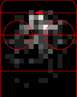
Where players shoot, however is even more interesting. I've initially looked at the three basic things you can look at when you're analyzing shots: shots, goals and shooting percentage. Ok the picutres are a little crude, I wanted to do this quickly. You can see on the percentage diagram has a few shots that always go in (outside the offensive zone), these are likely empty net shots (or else I guess they catch the goalie off guard). In the percentage diagram you can see that players can score from far locations at the correct angle. You can also see that shots closer to the net go in much more frequently. The shot diagram (the second one) it shows how many shots a location gets relative to all other locations. What I find interesting is how evenly distributed the shots are, yet shots from a certain distance have very bad odds of going in the net. In the third diagram I have goals (with the same relative "base" as shots), what I noticed is the 45^o line that goes along the left and a little along the right. On the left it goes over 30' to maybe 40' or so. You can see more goals seem to be scored on the right side of the net over the left.

I haven't really looked too much into this data and I only have around 5000 shots meaning this data isn't very accurate, but this looks promising so long as CBS continues publishing this data (and doesn't kill me for using it).

Standings

One thing that’s always fun to do is predict hockey games. HockeyAnalysis.com has developed a neat little prediction pool. Predicting from the first few games is hard you get a lot of error, plus teams can get unlucky with their starting opposition, making the data quite erroneous. That being said there are a number of ways to looking at the present data to figure out who’s the best team. One could use a rank system like Sagarin Ratings. I want to keep this simple and so I’ll look only at the standard Pythagorean prediction: gf²/ (gf²+ga²).

I’m not 100% satisfied with goals for, because it’s not all controlled by the one team, just because you don’t get goals doesn’t me you shouldn’t have gotten goals. Buffalo got 9 goals for against Philadelphia, shouldn’t be worth the same as 1 goal for against Anaheim. There are a number of options, but what I like to look at is expected goals for as it factors out the opponents goalie (but not their defense). Expected goals are not always the best indicator as offense, due to the fact there are a few (marginal amount) of players who can out score their expectations on a consistent basis, however it is much closer to offense than just goals for so I’ll use that as my goals for. I should qualify my use of these expected goals as there are only statistical estimates of goals and not actual goals. In fact if you compare these numbers to actual goals you’ll see:
that they match the expected error of ±15 (95% Confidence interval: [-30, 30]). This doesn’t indicate that expected goals for have no error themselves, but should indicate the error is smaller than the error with goals for and that’s why it’s a useful measure. The expected error for expected goals for per game is: √(3600*SFPG/3600*(1-SFPG/3600))*0.092 = 0.5 goals per game.

Defense is much more complicated to measure accurately, as mentioned above if a 9-1 game occur early in the season the teams’ statistics defensively are heavily affected by those 9 goals against and as such will likely appear worse than they really are. One cannot look at expected goals against, because they ignore the quality of the goaltending they have. So I’m stuck using standard goals against. As above you can estimate the error as √(3600*GAPG/3600*(1-GAPG/3600)) = 1.58 goals per game (remember that there are around 2.5 goals per game or that’s 63% of goals scored). Take note that expected goals for are three times more accurate than goals.

You can use addition and subtraction rules for values with standard deviation as well as for multiplication and division to get the error for an average team (50%):

GF²: √(2*(0.5/2.5)²)*2.5² = 1.76
GA²: √(2*(1.58/2.5)²)*2.5² = 5.58
GF² + GA²: √(1.76² + 5.58²) = 6.12 (or 12 ± 6)
GF²/(GF² + GA²): √( [6.12/(2*2.5²)] ² + [1.76/(2.5²)] ²)*0.5 = 0.36.

Now in order to implement this error estimate for higher winning percentages (I want linear) I need a method that doesn’t predict a team will win more than 100% of the time or lose more than 0% of the time that has the above error. This can be seen in the little graph.

Now I’m not going to show this, but binomial error decreases at √(n)/n (or 1/√(n)), where n is the number of games played. The same approximations can be made above and you get a decreasing winning percentage error as teams play more games. So I now have an error estimate as well as the winning percentages. Using the Poisson toolbox and I can get a prediction for every game based on goals for and against and then I can apply the above error rules to appropriately distribute the errors.

Note all these calculations are assuming that the teams do not change, which is in fact not true, because of injury and trades, but it’s the best estimate.

Now that you know how I’m determining who wins and loses each game I can now explain how I came up with my predictions. In order to get a average I need to cycle through the calculations below 10,000 times (take 45 minutes), I could do more, but I calculated the error to be around 0.5%, or probably around 1 point so 10,000 is a good balance between time and accuracy. I want to know 3 things: expected points, probability of making playoffs and probability of winning division.

First thing I calculate a random value for how much better or worse a team could be using the normal distribution and using the number of games played as a scale factor to lower the error to appropriate values. In order to calculate the error for an individual game I scale the linear errors from the teams to non-linear win prediction error (min: 0, max 1), following the concept of the little graph above, so games with a high probability of being wont are more likely be shifted down and similarly games with a low probability of being won are shifted up a little. However, most games (between 30% and 70%) are not affected at all by these things estimates as they are very close to linear. It should be clear that I look at every game individually so teams schedule difficulty are included in this estimate.

So no one care how I get there, but I now I have predictions for making the playoffs and winning the division many people remember from the end of last season. Here are the results for the west and for the east. You can see there are a number of teams with over and under estimate still, and that some teams have performed so bad that this system never predicts them in the playoffs.

Relative Face-off Scores.

Face-offs occur about as frequently as shots in a game. Just because there are many face-offs doesn’t mean they are extremely important, however, face-offs are a simple win loss game and as such allow a certain amount of simplified analysis. I’m sure there are many algorithms out there to do all this stuff for me, but I’m going to build this model from the ground up and keep it simple. Of course face-offs are a complicated dynamic between forwards and even at times defenseman to get the puck from a random dropping by a referee, but for now we are only going to be looking at one forward: the center.

Joe Thornton won at 52.3% in Boston and 50.1% in San Jose; he’s the same player why should the score differ so much? There are many reasons, but the most basic explanation is Joe Thornton got easier face-offs in Boston compared to San Jose. The idea is simple a player who gets easier opposition should get a better face-off percentage than average, but when he plays against good opposition he will perform much worse. Of course for face-offs opposition averages out quite nicely so most players are within a percentage point of the actual average. Of course it isn’t perfect as Sillinger performed at 52.6% in St. Louis, but at 55.0% in Nashville.

Theory

So how does one go about doing the calculations? Well, each team has around 4 regular face-off men, so there are around 120 guys (actually I did 121) I need to simultaneously compare in order to know who the best is. Before we can compare players we have to have an idea of who should win given some score of each player. What I really care about is the players “real” winning percentage, which should be approximately, be the win percentage vs. a 50% opposition and no player can win more than 100% of the time or lose more than 0% of the time. I’ll hand wave here, that the best two variable function to predict the odds of winning with two “players” is a Pythagorean prediction often used with runs scored in baseball or goals for and against in hockey.

p_a - probability of player 1 winning average
p_b - probability of player 2 winning average
p_ab = p_a²/(p_a²+p_b²)^*
p_ba = p_b²/(p_b²+p_a²)^*
FO_ab – face-offs between player 1 and player 2
FW_ab – face-offs wins by player 1 vs. player 2.

There are a few important relationships here that I should mention, these should be obvious, but I want to make them very clear to begin with

FO_ab = FO_ba
FW_ab= FO_ab * p_a²/(p_a²+p_b²)
FW_ba= FO_ab * p_b²/(p_b²+p_a²)

The above assumption is that the actual face-offs wins equals the prediction is required for this model, this isn’t quite true because of the error associated with the cross face-offs for many players is extremely high (only around 10 cross face-offs), but in general these problems “should” average out. So what I’m trying to do is solve for all the p_b and p_a information (there are up to n p’s), and I know how well each player did against every other player (n² - n – number of cross face-offs [-n because players can’t have face-offs against themselves]). Since we have FO_ab and FW_ab, I can easily calculate p_ab. FW_ab/FO_ab = p_ab, = p_a²/(p_a²+p_b²). This can be re-written as FO_ab* p_a² = FW_ab*(p_a²+p_b²) and there are n² equations just like it (Where FO_aa = 0). If you sum up n of them (fix a, change b) you get (where i goes from 1 to N):

Σ FO_ai* p_a² = Σ FWai*p_a²+ Σ FWai*p_b²
Or
Σ FO_ai* p_a² – Σ FW_ai*p_a² – Σ FW_ai*p_i² = 0
The nice thing is that this is equivalent to:
– Σ FL_a*p_a² + Σ FW_ai*p_i² = 0

There are N equations like this with N unknowns (p_i²’s). If you consider the p_i²’s as a variable without the power (eg. p_i² = c_i) as both are technically just constants. Then this problem is a linear system of N equations and N unknowns, however the solution is not unique, since the system is homogenous (there are infinitely many solutions, one of which is trivially all values are zero). How one solves this matrix is reasonably irrelevant, it’s reasonably large (121 x 121), but the solution will be the same no matter how you do it. I solved of this matrix by assuming a value for s, to get a b vector so I have an equation of Ax = b format, which I then solve using the “trivial” LU factorization or LUx = b. But, all you need to know is this matrix is solvable. Since it’s has N equations and N unknowns (and the matrix is non-singular) you actually get a set of solutions that is a vector multiplied by any constant (call this constant s) as a solution. In order to fix a solution I need a constraint for this constant. So I use the fact that that there were only so many face-offs between these players and their wins summed together must be equal to the total number of face-offs. Or Σ FO_i*p_i = Total Face-offs, where we know p_i² = c_i = b_i*s

Σ FO_i*s*b_i = Total Face-offs. (Know everything except s).
Total Face-offs/ Σ FO_i*b_i = s
Once I have s:
p_i = sqrt(b_i*s), and I’m done.

What I have just explained is how to simultaneously compare N players in the face-off circle. It’s hard to really understand what’s going on if you don’t deal with this sort of math on a regular basis; it took me a while to even come up with how to do it. You can easily make up trivial examples (each players takes 100 face-offs, 50 against each player) (the p_i² are the unknowns, A is the matrix in the equation Ax = 0.

FLa*pa2	FWab*pb2	FWac*pc2	= 0	A =	-45	26	29
FWba*pa2	FLb*pb2	FWbc*pc2			24	-51	25
FWca*pa2	FWcb*pb2	FLc*pc2			21	25	-54

What you should notice is that for example that 29 + 21 = 50 that the columns sum to 0. The positive numbers in the rows are that player’s wins and the negative numbers are the player’s losses. You’ll find s = 0.223 for the above example and the b_a = (2129/1671) and b_b = (607/557) and the last value b_c = 1 (by my choice in order to solve system) so

p_a = sqrt(0.223 * 2129/1671) = 0.5336 = 53.4%
p_b = sqrt(0.223 * 607/557) = 0.4935 = 49.4%
p_c = sqrt(0.223 * 1) = 0.4728 = 47.3%

These numbers don’t vary significantly from their original numbers (55%, 49% and 46%), but they’re different and on a bigger problem this can produce interesting results.

The Actual Results

Ax=0 system FW/(FW+FL) 1 Perreault, Y 63.75% Perreault, Y 62.18% 2 Vermette, A 58.78% Nieuwendyk, J 59.4% 3 Draper, K 57.98% Brind'amour, R 59.06% 4 Nieuwendyk, J 57.45% Vermette, A 57.9% 5 Brind'amour, R 57.04% Draper, K 57.73% 6 Malhotra, M 56.9% Stoll, J 56.75% 7 Johnson, R 56.41% Sillinger, M 56.64% 8 Yelle, S 56.04% Malhotra, M 56.35% 9 Mcdonald, A 55.38% Wellwood, K 56.32% 10 Sillinger, M 55.03% Mcdonald, A 56.23% 11 Johnson, G 54.62% Johnson, R 55.89% 12 Drury, C 54.57% Holik, B 55.67% 13 Halpern, J 54.44% Drury, C 55.51% 14 Peca, M 53.82% Yelle, S 55.41% 15 Holik, B 53.81% Sillinger, M 55.33% 16 Wellwood, K 53.58% Halpern, J 55.23% 17 Sundin, M 53.48% Johnson, G 54.92% 18 Stoll, J 53.4% Peca, M 54.87% 19 Green, T 53.38% Bergeron, P 54.66% 20 Smithson, J 53.33% Green, T 54.41% 21 Bergeron, P 52.94% Smithson, J 54.32% 22 Horcoff, S 52.67% Iginla, J 54.16% 23 Sillinger, M 52.67% Sundin, M 54.01% 24 Fedorov, S 52.61% Koivu, S 53.75% 25 Koivu, S 52.47% Cammalleri, M 53.46% 26 Wilm, C 52.45% Betts, B 53.33% 27 Marchant, T 52.44% Scatchard, D 53.2% 28 Handzus, M 52.22% Handzus, M 53.19% 29 Comrie, M 52.2% Datsyuk, P 53.07% 30 Cammalleri, M 52.1% Pahlsson, S 52.98% 31 Iginla, J 52.03% Comrie, M 52.75% 32 Hrdina, J 52.02% Horcoff, S 52.71% 33 Chouinard, M 51.96% Chouinard, M 52.71% 34 Sakic, J 51.88% Gomez, S 52.58% 35 Pahlsson, S 51.87% Spezza, J 52.55% 36 Scatchard, D 51.79% Sakic, J 52.49% 37 Betts, B 51.78% Reasoner, M 52.48% 38 Gratton, C 51.42% Wilm, C 52.31% 39 Taylor, T 51.28% Cullen, M 52.26% 40 Gomez, S 51.2% Thornton, J 52.25% 41 Spezza, J 51.03% Gaustad, P 52.23% 42 Bates, S 50.98% Taylor, T 52.12% 43 Armstrong, D 50.82% Smith, M 51.95% 44 Datsyuk, P 50.63% Hrdina, J 51.93% 45 Barnes, S 50.59% Fedorov, S 51.84% 46 Weight, D 50.57% Marchant, T 51.68% 47 Thornton, J 50.53% Dowd, J 51.66% 48 Smith, M 50.53% Savard, M 51.6% 49 Lang, R 50.39% Madden, J 51.52% 50 Madden, J 50.36% Bates, S 51.27% 51 Thornton, J 50.32% Gratton, C 51.25% 52 Roenick, J 50.23% Lecavalier, V 51.24% 53 Brown, C 50.22% Conroy, C 51.22% 54 Sedin, H 50.08% Arnott, J 51.15% 55 Primeau, W 50.03% Modano, M 51.09% 56 Conroy, C 50.01% Thornton, J 50.89% 57 Arnott, J 49.98% Armstrong, D 50.73% 58 Savard, M 49.97% Briere, D 50.68% 59 Lecavalier, V 49.91% Mclean, B 50.65% 60 Gaustad, P 49.9% Brown, C 50.62% 61 Modano, M 49.88% Forsberg, P 50.58% 62 Morrison, B 49.69% Sedin, H 50.52% 63 Briere, D 49.63% Morrison, B 50.41% 64 Begin, S 49.58% Lang, R 50.29% 65 Cullen, M 49.53% Fisher, M 50.28% 66 Yashin, A 49.5% Plekanec, T 50.28% 67 Zubrus, D 49.23% Zubrus, D 50.27% 68 Belanger, E 48.97% Zetterberg, H 50.26% 69 Cajanek, P 48.97% Richards, B 50.23% 70 White, T 48.96% Yashin, A 50.18% 71 Reasoner, M 48.93% Allison, J 50.11% 72 Mccauley, A 48.81% Begin, S 50.09% 73 Mclean, B 48.71% Barnes, S 50.08% 74 Fisher, M 48.62% Kapanen, N 49.87% 75 Zetterberg, H 48.51% Weight, D 49.84% 76 Allison, J 48.49% Primeau, W 49.8% 77 Linden, T 48.27% Smolinski, B 49.76% 78 Dowd, J 48.2% Laich, B 49.7% 79 Bell, M 48.17% Cajanek, P 49.66% 80 Plekanec, T 48.15% Linden, T 49.63% 81 Koivu, M 47.96% Roenick, J 49.44% 82 Richards, B 47.87% Ricci, M 49.21% 83 Ott, S 47.78% Stumpel, J 49.17% 84 Forsberg, P 47.76% Ott, S 49.16% 85 Reinprecht, S 47.74% Mccauley, A 49.13% 86 Sharp, P 47.71% White, T 49.1% 87 Smolinski, B 47.7% Belanger, E 49.02% 88 Stumpel, J 47.63% Adams, K 48.8% 89 Ricci, M 47.52% Brylin, S 48.7% 90 Langkow, D 47.41% Sutherby, B 48.67% 91 Mcclement, J 47.29% Turgeon, P 48.62% 92 Sutherby, B 47.16% Bell, M 48.45% 93 Brylin, S 46.88% Carter, J 48.17% 94 Carter, J 46.76% Sharp, P 48.04% 95 Goc, M 46.74% Roy, D 47.96% 96 Kesler, R 46.69% Goc, M 47.9% 97 Laich, B 46.63% Payer, S 47.57% 98 Jokinen, O 46.53% Koivu, M 47.38% 99 Adams, K 46.51% Rucchin, S 47.35% 100 Turgeon, P 46.33% Bonk, R 47.35% 101 Marleau, P 46.18% Langkow, D 47.35% 102 Kapanen, N 46.06% Reinprecht, S 47.34% 103 Payer, S 45.82% Jokinen, O 47.21% 104 Nylander, M 45.64% Walz, W 46.92% 105 Walz, W 45.33% Mcclement, J 46.89% 106 Legwand, D 45.28% Marleau, P 46.79% 107 Roy, D 45.21% Nylander, M 46.63% 108 Laperriere, I 45.05% Kesler, R 46.62% 109 York, M 44.64% Moore, D 46.49% 110 Kelly, C 44.57% Stefan, P 46.34% 111 Rucchin, S 44.53% York, M 46.08% 112 Stefan, P 44.5% Laperriere, I 45.9% 113 Moore, D 44.34% Kelly, C 45.75% 114 Ribeiro, M 44.11% Richards, M 45.73% 115 Bonk, R 43.9% Crosby, S 45.49% 116 Crosby, S 43.82% Ribeiro, M 44.72% 117 Connolly, T 43.81% Legwand, D 44.66% 118 Richards, M 43.78% Getzlaf, R 43.99% 119 Staal, E 42.21% Staal, E 42.89% 120 Getzlaf, R 41.76% Connolly, T 42.54% 121 Malone, R 39.22% Malone, R 39.56%

The whole point of of this was to prepare the skills I needed to do real analysis on shots for and against aka real icetime analysis. Looking at shot quality for an against for each player vs. every other player (Up to 1200 comparisons). So that's next!

* I used Pythagorean win percentage because it matched the properties I needed, I don’t think it’s perfect, but linear win prediction doesn’t work so you need something different.